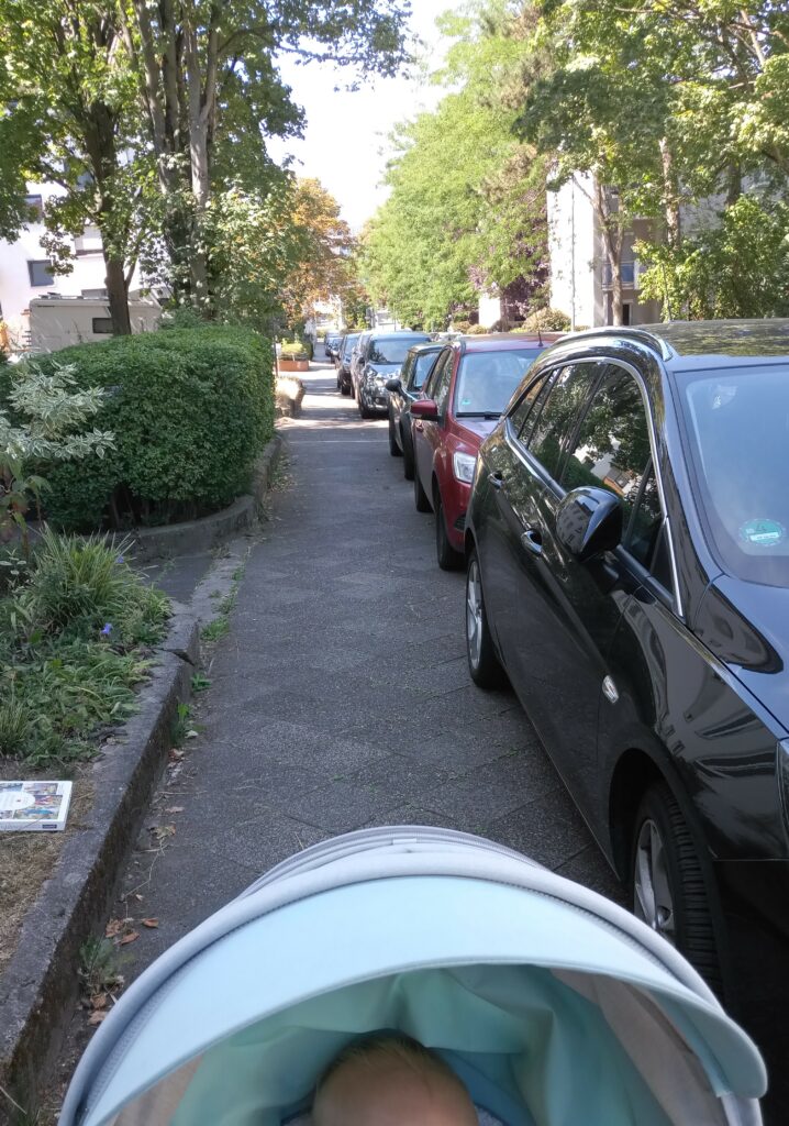
The annoyance by pavement and walkways blocked by parked cars has been rising again when I went back to parental leave with our second child. On the mere 900m from home to childcare, I was regularly blocked by parked cars despite the buggy only being 55cm wide.
The idea to measure and track the remaining width after motorists left their junk on/in my way grew already back in 2019. But there were always parts or time missing. Now finally, I am plugging together a little contraption that should be able to do what I want it to do: show and quantify how little space is left for pedestrians and how much of an obstacle this is to people who rely on small carts to help them move: parents, but also elderly with a walker or people in wheelchairs.
First things first: This is basically a remake of the famous OpenBikeSensor, which should – with a different firmware – totally work for this purpose, too. This is not about remaking the OBS. It’s rather a little write-up of what the process is about. And, of course, the proposal to use OBS or similar hardware to use for pavement width tracking (PWT, I guess I need a fancy three-letter shorthand 🤣).
The Sociopolitical Problem
For decades the city council of Darmstadt has simply tolerated parking on pavements. So much so that it is a very common sight in the city. This holds for many other German cities, too. But it causes trouble for pedestrians: You cannot walk next to each other, you can pass oncoming people only awkwardly (even more so during the pandemic), and finally if you’re trying to walk your baby to sleep or simply get somewhere with her or him, it’s close to scratching the sacred shiny finish of a car (Heil’ges Blechle) at best.
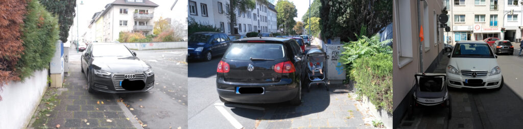
While the latter is an obvious problem (you’re blocked and have to cross the street or walk there), reporting such cases is a nuisance: call the #Unordnungsamt and if you’re lucky and someone picks up, they may come days later and instead of removing the car just fine the holder (the blocking car on the left was left in place for three days, the one in the middle for at least eight days). You can also report the car to the authorities. If you do that more often and happen to live in Bavaria, you risk a fine based on (imho grossly abused) data protection legislation (often being 8 times in the particular case). And then there are reports of city councils not going after the offenders even if presented with full evidence (at least this cannot be said for Darmstadt).
But the first, the constant abuse of pavement for parking, is indeed a problem. We have two push vehicles for our kids: one is a buggy (55 cm wide), one is a two seated bike trailer that works as buggy too (85 cm wide). Those are not excessive widths. The latter is about 15 cm wider than a wheelchair – though bear in mind that you need your hands to move the wheels, so 90 cm is consider the minimum passage width.
The hypothesis I want to prove with the BabyRanger (or any modified OBS) is: A large part of the public space is being obstructed by parked cars because pavement parking is tolerated.
The Technical Problem
Measuring distances ain’t easy. Estimating the distance between two obstacles left and right in a straight line, ideally perpendicular to either (at least one of) the obstacles’ surfaces, the walking direction and/or the footpath path direction is a different story still.
Other problems I can think of: Deciding which side of the street you are on. Whether you are blocked and have to change sides or simply wanted to cross the street. How to detect if the sensors are misplaced. How to install the system on the various kinds of carts there are. And so on…
Mapping those data in a geographically meaningful way without disclosing the whereabouts and routes of the user of the system, and how to visualise the whole thing, is a yet another story.
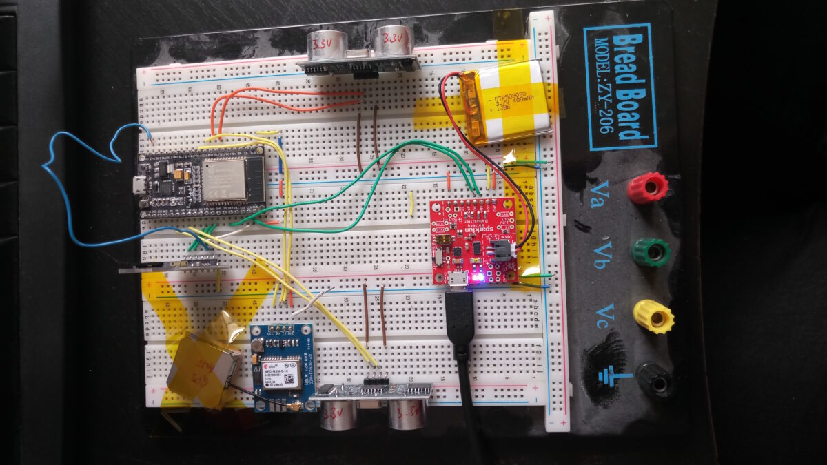
What I’m Currently Doing
At the moment all I am struggling with is the GPS module. I chose NeoGPS as framework and it’s powerful, but pretty easy to get lost in. At the moment, UART is doing its thing, the logic analyser can read meaningful data at the chosen settings too, and NMEA sentences are transmitted.
However, they only fill the buffer but don’t produce any fixes let alone position data.
So: I’m in between tinkering a little more or switching to a different framework.
[Update 2022-10-15]
Well, the 3.3V SD card breakouts arrived yesterday, so let’s go for a walk. Roughly 20 minutes (i.e. ~1200 seconds) and guess what this beauty scribbled to flash drive:
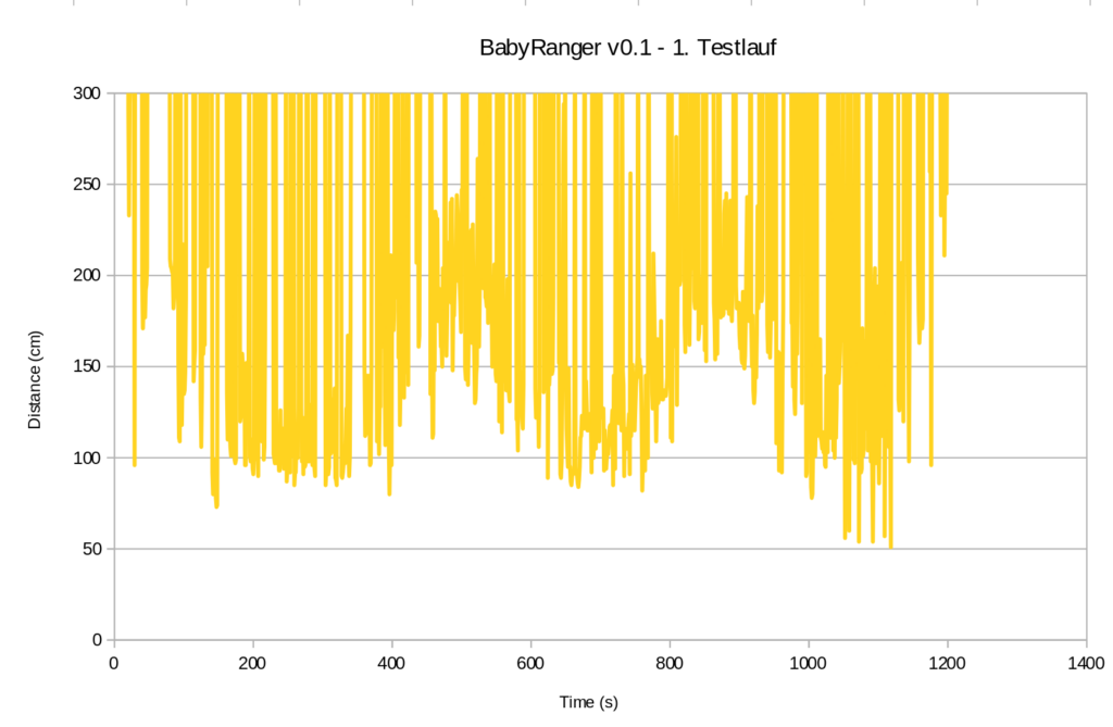
So, even though I would say it’s been a very tidy situation on the pavements (judging from experience in the street I walked down), here we go: Below 100 cm almost half the time and towards the end down to 50 cm. To be taken with a huge pinch of salt though until stuff like alignment, stability, unexpected obstacles etc. are properly taken care of.
[End of Update 2022-10-15]
Invitation
While I will be able to devote only limited time on this, I invite anyone with an OBS to see what solution they could think of. And to contact me if you’re interested to work on this issue ☟