SymPy

SymPy allows quick and (relatively 😜) easy manipulation of algebraic expressions. But it can do so much more! Using the sympy.physics.control toolbox, you can very inspect linear time-invariant systems in a very comfortable way.

I was looking at a paper (Janiszowski, 1993) which features three transfer functions of different properties and wanted to look at their pole-zero diagrams as well as their Bode plots in real frequency. The transfer functions where the following:

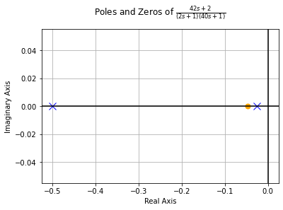
(1) $\begin{align*} G_1(s) &= \frac{ 2 + 42s }{ (1 + 2s)(1 + 40s) } \\ G_2(s) &= \frac{ 5 - 60s }{ (1 + 4s)(1 + 40s) } \\ G_3(s) &= \frac{ 4(1 + s) }{ 1 + 4s + 8s^2 } \end{align*}$

Drawing the pole-zero diagrams from this representation is easy:

Zeros: Set numerator to zero
Poles: Set denominator (or its individual terms) to zero

Drawing the Bode diagram however would’ve involved some basic programming. But neither is necessary.

import sympy as sy
from sympy.physics.control.lti import TransferFunction as TF
from sympy.physics.control import bode_plot, pole_zero_plot

s = sy.symbols("s", complex=True)

G1 = (2 + 42*s)/((1 + 2*s)*(1 + 40*s))
tf = TF(*G.as_numer_denom(), s)
bode_plot(tf)
pole_zero_plot(tf)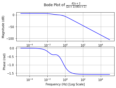

Bode plot of the transfer function G₁(s)

Pole-Zero diagram of the transfer function G₁(s)

Well, that was easy. TransferFunction (abbreviated with TF in my examples) requires numerator and denominator to be passed as separate arguments. sympy_expr.as_numer_denom() is convenient, as it returns a (numerator, denominator) tuple. Using the asterisk expands this.

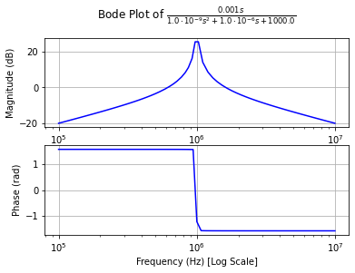
Now, what else can we do with this? Look at RLC resonators, for example:

A parallel resonator of resistance R, inductance L and capacitance C

The reactance of the inductor and capacitor are given by

(2) $\begin{equation*} X_C = \frac{1}{sC} \quad \text{and} \quad X_L = sL \end{equation*}$

where s is basically the complex frequency (we’re looking at this with Laplace eyes). Now, off to SymPy we go:

R, C, L = sy.symbols("R, C, L", real=True, positive=True)
Xc, Xl = 1/(s*C), s*L

def par(a, b):
    # Shorthand for a parallel circuit
    return a*b/(a+b)

G = par(Xc, par(R, Xl)).ratsimp()
G = G.subs({R: 1e3, L: 1e-6, C: 1e-6})
tf = TF(*G.as_numer_denom(), s)
bode_plot(tf, 5, 7)
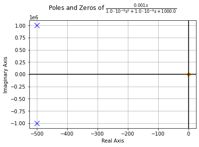
pole_zero_plot(tf)

For visualisation we choose R = 1 kΩ, L = 1 µH and C = 1 µF.

Bode plot of the parallel RLC circuit with R = 1 kΩ, L = 1 µH and C = 1 µF, and hence a resonance frequency of 1 MHz

And its pole-zero plot just for the lolz.

Why is this useful? Well, because it is quick and robust and once you have your transfer function typed out, you get the impulse and step responses for free:

import sympy as sy
from sympy.physics.control import impulse_response_plot
from sympy.physics.control import step_response_plot

s = sy.symbols("s", complex=True)
G1 = (2+42*s)/((1+2*s)*(1+40*s))
G2 = (5-60*s)/((1+4*s)*(1+40*s))
G3 = 4*(1+s)/(1+4*s+8*s**2)

for G in [G1, G2, G3]:
    tf = TF(*G.as_numer_denom(), s)
    bode_plot(tf)
    pole_zero_plot(tf)
    step_response_plot(tf, upper_limit=60)
    impulse_response_plot(tf, upper_limit=60)

Note: SymPy’s adaptive plotting is not particularly good at plotting oscillations, so the impulse response of the RLC circuit above will look ugly.