Category: Uncategorized

What the European Railways and the European Payment Area have in common

Post author By cweickhmann
Post date 2 September 2026

This is a short piece about what I think the two entities in the title have in common. And the way I found remarkably telling is through signing up to the European Rail Passengers Union, which by the way you should absolutely consider if you are using railways in Europe at all.

First things first: I wanted to sign up to the ERPU because I think they do crucial work to improve the passenger experience on rails in Europe – which sucks right now.

The ERPU is an association under Belgian law, you can sign up online for only 12€/year, and hey, in the payment process, amongst all the usual payment options, I get “iDEAL Wero”.

Wero you say? I can try this new European payment method? Nice! I’m hooked! So, I click.

And there’s a QR code saying “scan me with your banking app”.

Well. My banking app says, this is not a Wero link – and apparently it isn’t.

So I click on the other button that says: Or use internet banking, select your bank.

All right, so I click this.

And it lists … only Belgian banks.

So, what do I do? ~~I take the plane.~~ I pay using Visa/Mastercard/Amexco.

This is exactly what the European Rail experience is today:

You try. You try again. The connection is shoddy, you have no rights in case ticket 1 fails and you miss your train on ticket 2. ~~So, you use Paypal~~. So, you take the plane.

Here it’s the same. There’s this European payment service Wero, that in principle could be used Europe wide. But implementation on all sides – bank, service provider – is crappy. It’s limited to national borders for yet another completely in-transparent reason. And so, you pay using credit card.

And it’s probably for the exact same reasons too. Like train operators, many banks have their turf, are safe because they’re the default and somewhat state backed (yes, I’m looking at you Sparkassen) and haven’t adapted to demand in decades. Like train regulation, regulators only seem to care what’s going on when shit is on fire (cf. sub prime loan crisis et al., or railway tracks crumbling under twice the load they were constructed for et al.). And like in train land, there’s the other agile, indirectly but heavily subsidised means of payment with a shitload of hidden downsides that you default to. You don’t think cars and planes have massive downsides? Maybe you also think, Mastercard, Visa, PayPal and Apple/Google Pay offer their services for free. Heck no, you simply don’t ever see the bill. And: Yes, et al indeed.

And this is not a dunk on the folks at ERPU. On the contrary: they’ve taken what is available in terms of payment services, integrated it nicely into their web page. Jon is doing actual field work travelling around all the crazy cross border connections that barely work in Europe. No. The horror starts once you leave their web page and enter into the payment service realm.

But it illustrates so very clearly why it’s so bad. And why work like the one of ERPU is needed. Hell, maybe we need more than the European Rail Passenger Union. We need a European Payment Users Union. How’s that?

Uncategorized

The details of CAN with the STM32 toolchain

Post author By cweickhmann
Post date 17 February 2026

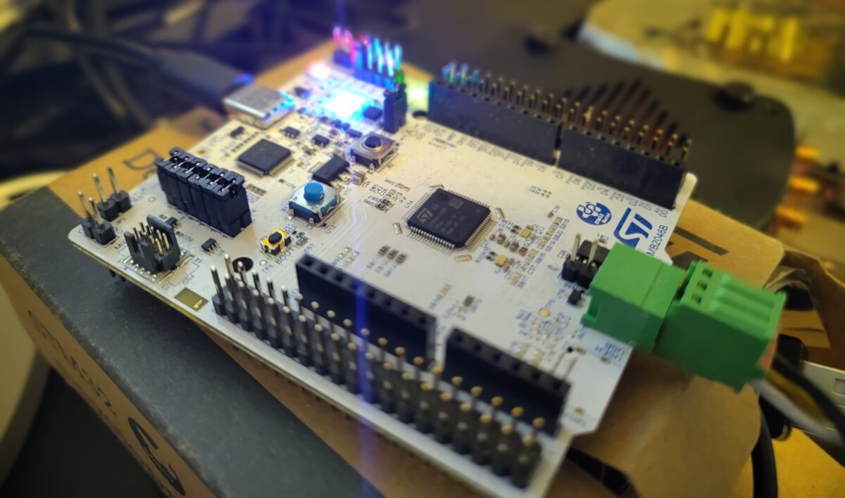
This is a blog entry about how sometimes you just get overwhelmed by UI and consequentially lost. I was looking into CAN on an STM32 dev board (the Nucleo C092RCT) when I ran into the strange issue that my little test programme would transmit CAN frames fine, but somehow not receive them.

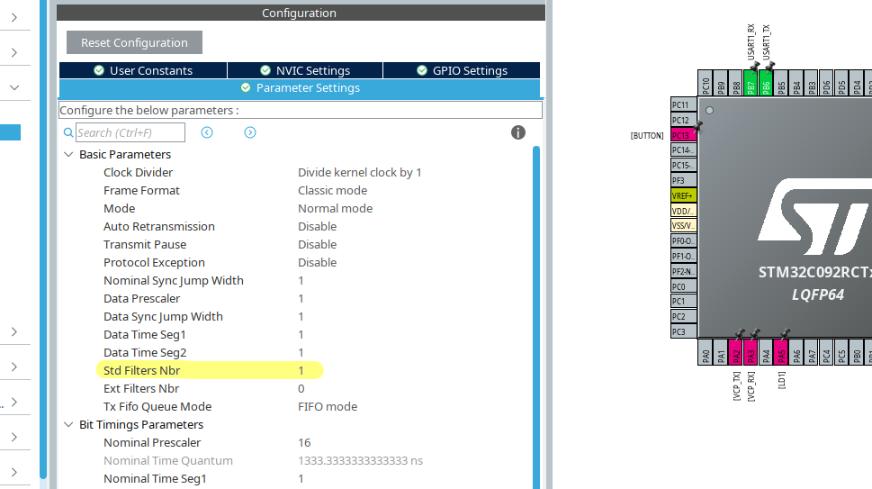
Searching forums did not return anything that solved my issue. I did find posts stating that in order for CAN to work, you’d have to set the number of filters to 1 (Std Filters Nbr).
While it is true, that you need this in order to filter by criteria like the identifier, having the filter number set to 0 simply lets everything pass and so the HAL should in theory respond to any message on the bus.

But since I wanted to filter by an ID, I set it anyway like so:

But then I though: “Let’s explore the UI of STM32CubeMX a bit more. And behold: There’s an interrupt tab called “NVIC Settings” that escaped my view before and FDCAN1 interrupt 0 is not enabled. Let’s change that like so:

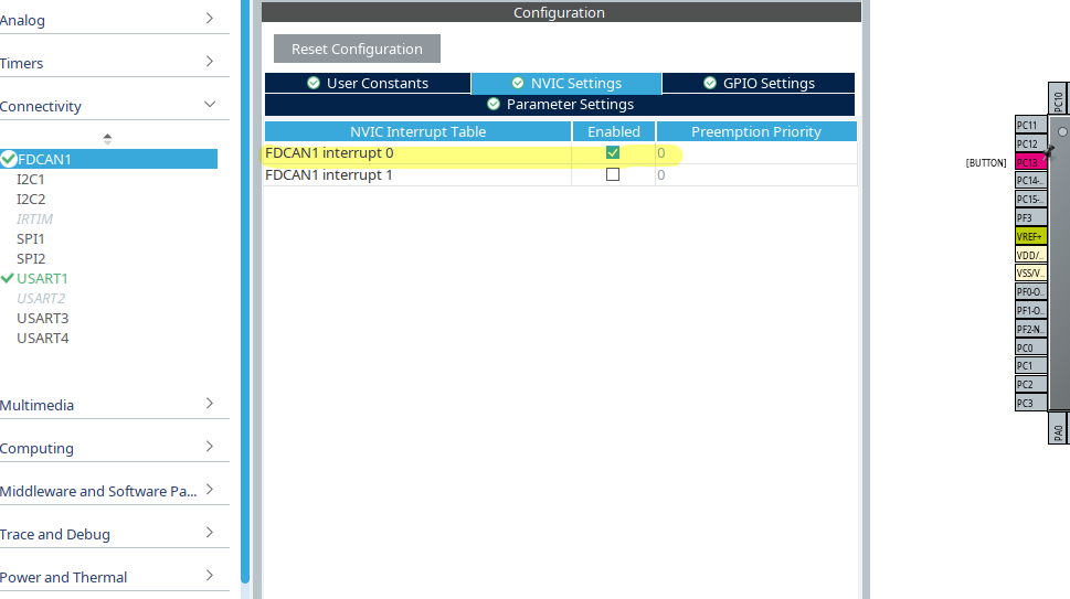
And would you know it: Now sending a CAN frame with appropriate Identifier would actually cause the callback function HAL_FDCAN_RxFifo0Callback to be called and toggle my little green LED.

Some forum posts claimed you’d need to configure global filters by invoking HAL_FDCAN_ConfigGlobalFilter. And that is actually true. What got me, however, is the FilterType, where I have to admit I do not understand the behaviour of two of the three options: FDCAN_FILTER_DUAL seems pretty clear to me, it passes what matches either of the two filter IDs given by FilterID1 and FilterID2. FDCAN_FILTER_MASK however evades me. I guess it’s something like ID1 corresponding to a positive and ID2 to a negative mask (iduno). What confused me a lot was FDCAN_FILTER_RANGE which did not behave at all as I thought (my though: ID1 is the lower and ID2 the upper boundary of the range).

So here’s the snippet that actually worked for me:

static void FDCAN_Config(void) {
  FDCAN_FilterTypeDef sFilterConfig;
  // Rx Filters
  sFilterConfig.IdType = FDCAN_STANDARD_ID;
  sFilterConfig.FilterIndex = 0;
  sFilterConfig.FilterType = FDCAN_FILTER_DUAL; // other options: FDCAN_FILTER_MASK, FDCAN_FILTER_RANGE
  sFilterConfig.FilterConfig = FDCAN_FILTER_TO_RXFIFO0;
  sFilterConfig.FilterID1 = 0x400;
  sFilterConfig.FilterID2 = 0x321;
  if (HAL_FDCAN_ConfigFilter(&hfdcan1, &sFilterConfig) != HAL_OK) Error_Handler();

  if (HAL_FDCAN_ConfigGlobalFilter(&hfdcan1, FDCAN_REJECT, FDCAN_REJECT, FDCAN_REJECT_REMOTE, FDCAN_REJECT_REMOTE) != HAL_OK) Error_Handler();

  // Start Module
  if (HAL_FDCAN_Start(&hfdcan1) != HAL_OK) Error_Handler();
  if (HAL_FDCAN_ActivateNotification(&hfdcan1, FDCAN_IT_RX_FIFO0_NEW_MESSAGE, 0) != HAL_OK) Error_Handler();

  // Prepare Tx
  TxHeader.Identifier = 0x321;
  TxHeader.IdType = FDCAN_STANDARD_ID;
  TxHeader.TxFrameType = FDCAN_DATA_FRAME;
  TxHeader.DataLength = FDCAN_DLC_BYTES_4;
  TxHeader.ErrorStateIndicator = FDCAN_ESI_PASSIVE;
  TxHeader.BitRateSwitch = FDCAN_BRS_OFF;
  TxHeader.FDFormat = FDCAN_CLASSIC_CAN;
  TxHeader.TxEventFifoControl = FDCAN_NO_TX_EVENTS;
  TxHeader.MessageMarker = 0;
}

void HAL_FDCAN_RxFifo0Callback(FDCAN_HandleTypeDef *hfdcan, uint32_t RxFifo0ITs) {
  if ( (RxFifo0ITs & FDCAN_IT_RX_FIFO0_NEW_MESSAGE) != RESET) {
  if (HAL_FDCAN_GetRxMessage(hfdcan, FDCAN_RX_FIFO0, &RxHeader, RxData) != HAL_OK) Error_Handler();
    BSP_LED_Toggle(LED_GREEN);
    printf("HAL_FDCAN_RxFifo0Callback! %s\r\n", (char*) RxData);
}

I hope, this helps some. By the way: If you play with options in STM32CubeMX, double check the other options – they tend to get reset as you play with other values.

Uncategorized

Using Sympy’s Common Subexpression Elimination to generate Code

Post author By cweickhmann
Post date 8 March 2024

A nifty feature of sympy is its code generator. This allows generating code in many languages from expressions derived in sympy. I’ve been using this for a while and came across the Common Subexpression Elimination (CSE) function (again), recently.

In earlier* versions of sympy I did not find it of great use. But now I was pleasantly surprised how much it matured. (* I cannot say for sure when I last tried using it; it must’ve been a long while ago.)

What is it and what is it good for?

Let’s say we want to generate code for a PI controller in C. The literature says its transfer function (in DIN notation) reads:

$G(s) = K_p + \frac{K_i}{s}$

Then furthermore the representation for a discrete time system with time step $T_s$ becomes

$G(z) = K_p + \frac{K_i T_s}{2} + \frac{\frac{K_i T_s}{2} - K_p}{z}$

In order to efficiently and flexibly calculate the response we want to implement it in a second order IIR (infinite impulse response) filter structure. This structure is basically a representation of $G_z$ as a rational function

$\frac{ b_0 + b_1 z^{-1} + b_2 z^{-2} }{ a_0 + a_1 z^{-1} + a_2 z^{-2} }$

so we need to take the expression apart such that we can determine the coefficients a_1, a_2, b_0, … (by convention, the problem is scaled such that a_0 = 1.

This is all very cumbersome to do manually (and I suck at doing this, especially as I insert quite embarrassing mistakes all the time). So, sympy to the rescue:

import sympy as sy

Kp, Ki, Ts = sy.symbols("K_p K_i T_s", real=True)
z = sy.symbols("z", complex=True)
G_z = Kp + Ki*Ts/2 + (Ki*Ts/2 - Kp)/z

display(G_z)

n, d = G_z.ratsimp().as_numer_denom()
n, d = n.as_poly(z), d.as_poly(z)

display(n, d)

We first define the symbols needed. Then set up G_z according to our equation above. After displaying it for good measure, we do a rational simplification ratsimp() on it and split it into numerator n and denominator d.

Now, we represent n and d as polynomials of z. And this is how we obtain our coefficients a1, a2, and so on. We continue:

scale = d.LC()

n, d = (n.as_expr()/scale).as_poly(z), (d.as_expr()/scale).as_poly(z)
N, D = n.degree(), d.degree()

We find the scaling factor as the leading coefficient (LC()) of the denominator d, scale both accordingly and determine the degree of each (this is mostly to determine for how many terms we have to iterate when printing etc.).

Bs = n.all_coeffs()
As = d.all_coeffs()

display(Bs)
display(As)

Now, basically Bs contains all coefficients [b0 b1] and likewise for As. Here’s a shortcut, see if you can spot it.

And now comes the cse magic:

commons, exprs = sy.cse(Bs)

This returns a tuple. The first element is a list of tuples of arbitrarily assigned place holder variables x0, x1, and so on. The second element are the original expressions, but the placeholders are substituted. In this example:

(
  [
    (x0, K_i*T_s/2)
  ],
  [K_p + x0, -K_p + x0]
)

Which means, instead of calculating K_i*T_s/2 twice, we can do it once, assign it to x0 and use that on the expressions.

You can even concatenate As and Bs for good measure (not really necessary here, since the As only contain 1 and 0, but in other controller topologies this may change).

commons, exprs = sy.cse(As + Bs)

# Printing C code for instance
for com in commons:
    print( sy.ccode(com[1], assign_to=repr(com[0])) )

for expr, name in zip(exprs, "a0 a1 b0 b1".split(" ")):
    print( sy.ccode(expr, assign_to=f"coeffs.{name:s}") )

We obtain the common terms commons and the reduced expressions exprs, then print the common terms assigning them to their respective placeholder variables, and finally print the reduced expressions. This produces this five liner in C:

x0 = (1.0/2.0)*K_i*T_s;
coeffs.a0 = 1;
coeffs.a1 = 0;
coeffs.b0 = K_p + x0;
coeffs.b1 = -K_p + x0;

Now, how is this useful you ask? Well, for this toy example it certainly is a lot of work for five lines I could’ve just typed out.

But if you go into a PID controller with damped differential term, and you want your code to be efficient (i.e. have as few operations as possible), this is very handy. Just by changing the symbols and the expression for G_z we obtain this:

x0 = 2*T_v;
x1 = 1.0/(T_s + x0);
x2 = 4*T_v;
x3 = T_i*T_s;
x4 = 2*x3;
x5 = T_i*x2;
x6 = 1.0/(x4 + x5);
x7 = K_p*x4;
x8 = K_p*T_s*x0;
x9 = pow(T_s, 2);
x10 = 4*K_p*T_d*T_i + K_p*x5;
x11 = K_p*x9 + x10;
c.a0 = 1;
c.a1 = -x1*x2;
c.a2 = x1*(-T_s + 2*T_v);
c.b0 = x6*(x11 + x7 + x8);
c.b1 = (K_p*x9 - x10)/(T_i*x0 + x3);
c.b2 = x6*(x11 - x7 - x8);

I did this manually once, and only obtained five or six of the placeholders. That’s the power of cse().

Oh, you need the code in Python for testing? No problem, just use pycode instead (and work around that assign_to parameter).

So, there you have it.

Uncategorized

Got a R&S FSH4 and want to extract screenshots?

Post author By cweickhmann
Post date 7 July 2022

Situation: I’ve taken about 50ish measurements on an FSH4 spectrum analyser saving a dataset of each using the save data function of the spectrum analyser.

Turns out: The R&S InstrumentView application does not install on Wine. So, how do I get the screenshots embedded in the saved datasets? Right: Search for the PNG magic number and a chunk end.

This is really sketchy but worked on all measurement files. If you’re in the same situation, just check out my repository.

https://gitlab.com/cweickhmann/extract-png-from-rs-set

Note: No affiliation with R&S whatsoever. Please don’t pester them if the script is not working.

Tags measurement, png, python, spectrum analyser

Linux Uncategorized

Lost Gitea Local Admin Password?

Post author By cweickhmann
Post date 26 April 2022

There are various possible ways you can lose access to your Gitea instance. In particular, if you are getting user accounts via LDAP, you should always have a key to get back in: a “local” admin.

In case you haven’t got one (totally not like I did definitely only once 🤫), deleted it or lost its password, here’s the procedure in to variants: running on plain Linux, and running within Docker.

Plain Linux

List the available (local) user accounts (you may need to run this with sudo):

$ gitea admin user list

ID   Username     Email             IsActive IsAdmin
1    user1        me@home.earth     true     false

You may not get a single user listed here. In order to add a local administrator, do this

$ sudo gitea admin user create --username local_admin --email admins@email.earth --admin --random-password

generated random password is 'IzgvOwv1M9EG'
New user 'local_admin' has been successfully created!

$ sudo gitea admin user list

ID   Username     Email                 IsActive IsAdmin
1    unpriv_local bowfingermail@gmx.net true     true
3    local_admin  admins@email.earth    true     true

Especially on shared machines, I’d strongly recommend not setting a password via the command line. It’ll stick in bash_history and may be visible in the process list. Hence the --random-password option here. Use the generated password upon first login in the browser.

Docker Container

In order to get to the “plain Linux” field, you simply run a bash in the Gitea Docker container.

What’s the container’s name? Get it via docker container ls -a. Let’s say it’s called gitea. To start bash in that container, do

user1@linux:$ docker exec -it gitea /bin/bash

Now, you basically do the same thing as in the section above.

docker # gitea admin user list

ID   Username     Email             IsActive IsAdmin
1    user1        me@home.earth     true     false

docker # gitea admin user create --username local_admin --email admins@email.earth --admin --random-password

generated random password is 'ikV6xzPTiH7B'
New user 'local_admin' has been successfully created!

docker # gitea admin user list

ID   Username     Email                 IsActive IsAdmin
1    unpriv_local bowfingermail@gmx.net true     true
3    local_admin  admins@email.earth    true     true

Conclusion (and Other Platforms)

The Plain Linux approach works equally well on other platforms. I hope this helps.

Tags admin, docker, gitea, Linux

Uncategorized

Numbers games: Z-Transform and some sympy

Post author By cweickhmann
Post date 25 April 2022

Back in uni me and control systems never really clicked. So I took a dive into the topic as I had the time. Long story short for all who know equally little or even less about the maths of control systems as I do:

Often, you model control systems using the Laplace transform. That’s nice and good for continuous systems.
Once you’re going to the discrete (digital) world, you want to use the Z-transform.
There is a (complicated) relation between Laplace domain and Z domain.
There are approximations, using a complex maps to map from Laplace to Z domain (a bilinear transformation, Tustin’s method, being the one used here).

This is a post on serendipity, because what this is about is actually neither control systems, Z-, or Laplace transforms but a numbers game. Bare with me.

Many systems can be modelled using a rational function of the form

$G(s) = \frac{\sum\limits_{i=0}^m \beta_i s^i}{\sum\limits_{i=0}^n \alpha_i s^i} \qquad\text{\alpha_0 = 1}$

You can easily put this into sympy and play around with it.

import sympy as sy

s, z, Ts = sy.symbols("s, z, T_s")

a0 = sy.S.One
a1, a2 = sy.symbols("alpha_1, alpha_2")
b0, b1, b2 = sy.symbols("beta_0, beta_1, beta_2")

G = (b0 * s**2 + b1 * s + b2) / (a0 * s**2 + a1 * s + a2)
G # use `print(sy.latex(G))` to get the LaTeX representation

$\frac{\beta_{0} s^{2} + \beta_{1} s + \beta_{2}}{\alpha_{1} s + \alpha_{2} + s^{2}}$

Nice. Let’s generalise this a little bit:

import sympy as sy

s, z, Ts = sy.symbols("s, z, T_s")

N, M = 2, 2

a = sy.symbols(f"alpha_1:{N+1}")
a = (sy.S.One, *a)
b = sy.symbols(f"beta_0:{M+1}")

G = sy.Add(*[b[i] * s**i for i in range(M+1)]) / sy.Add(*[a[i] * s**i for i in range(N+1)])

By playing with the values for N and M we can now generate any order of rational function we wish. Again, not the thing this article is about.

Then there is the bilinear transform called Tustin’s method that approximately maps the function G from the Laplace domain into the Z domain.

$s \Rightarrow \frac{2}{T_s} \frac{z-1}{z+1}$

Let’s do this in sympy:

tustin = 2/Ts * (z-1)/(z+1)

G.subs({s: tustin}).simplify()

$\frac{T_{s}^{2} \beta_{0} \left(z + 1\right)^{2} + 2 T_{s} \beta_{1} \left(z - 1\right) \left(z + 1\right) + 4 \beta_{2} \left(z - 1\right)^{2}}{T_{s}^{2} \left(z + 1\right)^{2} + 2 T_{s} \alpha_{1} \left(z - 1\right) \left(z + 1\right) + 4 \alpha_{2} \left(z - 1\right)^{2}}$

Sweet. Now, I want to have the representation in two polynomials in z (numerator and denominator) to extract the coefficients (because that’s what I wanted to hack into code):

num, den = G.as_numer_denom()
num = sy.Poly(num, z)
den = sy.Poly(den, z)

num.coeffs()
den.coeffs()

This gives you a nice, codeable result:

num: [  T_s**2*beta_0 + 2*T_s*beta_1  + 4*beta_2,
      2*T_s**2*beta_0                 - 8*beta_2,
        T_s**2*beta_0 - 2*T_s*beta_1  + 4*beta_2]
den: [  T_s**2        + 2*T_s*alpha_1 + 4*alpha_2,
      2*T_s**2                        - 8*alpha_2,
        T_s**2        - 2*T_s*alpha_1 + 4*alpha_2]

… but my eye spotted a pattern here. Do you see it? It’s easier to see in matrix representation, and I’ll only look at num (i.e. the expression with β_i in it, because I set ɑ₀ to 1):

$\text{num}^{(N=2)} = \begin{pmatrix} 1 & +2 & +4 \\ 2 & 0 & -8 \\ 1 & -2 & +4 \end{pmatrix} \cdot \begin{pmatrix} T_s^2 \beta_0 \\ T_s^1 \beta_1 \\ T_s^0 \beta_2 \end{pmatrix}$

Here is the resulting matrix for N = M = 3 and for N = M = 5:

$\text{num}^{(N=3)} = \begin{pmatrix} 1 & 2 & 4 & 8 \\ 3 & 2 & -4 & -24 \\ 3 & -2 & -4 & 24 \\ 1 & -2 & 4 & -8 \\ \end{pmatrix} \cdot \begin{pmatrix} T_s^3 \beta_0 \\ T_s^2 \beta_1 \\ T_s^1 \beta_2 \\ T_s^0 \beta_3 \end{pmatrix} \\ \text{num}^{(N=5)} = \begin{pmatrix} 1 & 2 & 4 & 8 & 16 & 32 \\ 5 & 6 & 4 & -8 & -48 & -160 \\ 10 & 4 & -8 & -16 & 32 & 320 \\ 10 & -4 & -8 & 16 & 32 & -320 \\ 5 & -6 & 4 & 8 & -48 & 160 \\ 1 & -2 & 4 & -8 & 16 & -32 \end{pmatrix} \cdot \begin{pmatrix} T_s^5 \beta_0 \\ T_s^4 \beta_1 \\ T_s^3 \beta_2 \\ T_s^2 \beta_3 \\ T_s^1 \beta_4 \\ T_s^0 \beta_5 \end{pmatrix}$

Here are the resulting matrices for N = M = 4:

$\text{num}^{(N=4)} = \begin{pmatrix} 1 & 2 & 4 & 8 & 16 \\ 4 & 4 & 0 & -16 & -64 \\ 6 & 0 & -8 & 0 & 96 \\ 4 & -4 & 0 & 16 & -64 \\ 1 & -2 & 4 & -8 & 16 \end{pmatrix} \cdot \begin{pmatrix} T_s^4 \beta_0 \\ T_s^3 \beta_1 \\ T_s^2 \beta_2 \\ T_s^1 \beta_3 \\ T_s^0 \beta_4 \end{pmatrix}$

Here are the resulting matrices for N = M = 6

$\text{num}^{(N=6)} = \begin{pmatrix} 1 & 2 & 4 & 8 & 16 & 32 & 64 \\ 6 & 8 & 8 & 0 & -32 & -128 & -384 \\ 15 & 10 & -4 & -24 & -16 & 160 & 960 \\ 20 & 0 & -16 & 0 & 64 & 0 & -1280 \\ 15 & -10 & -4 & 24 & -16 & -160 & 960 \\ 6 & -8 & 8 & 0 & -32 & 128 & -384 \\ 1 & -2 & 4 & -8 & 16 & -32 & 64 \end{pmatrix} \cdot \begin{pmatrix} T_s^6 \beta_0 \\ T_s^5 \beta_1 \\ T_s^4 \beta_2 \\ T_s^3 \beta_3 \\ T_s^2 \beta_4 \\ T_s^1 \beta_5 \\ T_s^0 \beta_6 \end{pmatrix}$

The odd values for N and M produce matrices with all non-zero values, so I’ll look at those first.

What I find stunning is the fact that there are so many patterns and yet I fail to think of a pattern that creates the whole matrix. For example, the first column clearly follows the binomial distribution:

$\begin{pmatrix}N \\ k\end{pmatrix}$

where k is the row number starting with 0.

The first and last rows of the matrix are power series of 2 and -2 respectively:

$2^l \quad \text{and} \quad (-2)^l$

where l is the column number starting at 0.

Every column has a different sign pattern starting at all positive on column 0 and alternating, starting with + on the last column.

Ignoring the signs, the columns are related like this

N	#0 ↷ #N-1	#1 ↷ #N-2	#2 ↷ #N-3	#3 ↷ #N-4
3	྾ 8	྾ 2
5	྾ 32	྾ 8	྾ 2
7	྾ 128	྾ 32	྾ 8	྾ 2

What multiples relate the l^th column from the left with the l^th column from the right, ignoring the sign.

Maybe this follows from the power series mentioned earlier. But looking at the coefficients in each column the binomial pattern is lost as you move to the inside.

And last but not least wild zeros appear when you look at the even values for N and M:

Apparently, in the middle row as well as the middle column, every other value is zero.

All right, I’m absolutely sure mathematicians and control systems theoreticians have looked at this back in the day and this is all solved and done. Still, I found it interesting to look at.

If you want to create those values yourself, you can use this little script, and modify N and M. But beware, at N = 10 the script runs for 10 seconds.

import sympy as sy

s, z, Ts = sy.symbols("s, z, T_s")

N, M = 3, 3  # <-- Modify here

a = sy.symbols(f"alpha_1:{N+1}")
a = (sy.S.One, *a)
b = sy.symbols(f"beta_0:{M+1}")

G = sy.Add(*[b[i] * s**i for i in range(M+1)]) / sy.Add(*[a[i] * s**i for i in range(N+1)])

tustin = 2/Ts * (z-1)/(z+1)
G = G.subs({s: tustin}).simplify()

num, den = G.as_numer_denom()
num = sy.Poly(num, z)
den = sy.Poly(den, z)

for l in num.coeffs():
    p = sy.Poly(l, Ts)
    for i, B in enumerate(p.all_coeffs()):
        try:
            coeff, _ = B.as_two_terms()
        except:
            coeff = 0 if B is sy.S.Zero else 1
        print(f"{repr(coeff):6s} & ", end="")
    print()

Oh, and of course you can change N and M independently from each other, but I could not be bothered to look at this as well.

Tags mathematics, numbers, sympy

Uncategorized

Rogue docker processes on Ubuntu: Snap!

Post author By cweickhmann
Post date 22 February 2022

I’ve come across a situation where out of three docker containers that should be running, only one was shown by docker container ls -a. Weird, hu?

The missing two were clearly running their processes because the web service they provided was active and reachable.

After a lot of forth and back, it turned out that Ubuntu 20.04 with snap came with a docker snap – and had a recent Docker CE installed via the apt package manager. Don’t do that.

Once the snap docker was removed, it worked and showed all the containers again.

Uncategorized

Missing important details: Don’t update to DSM 7 yet*

Post author By cweickhmann
Post date 15 November 2021

*) if you rely on the SynoCommunity package rdiff-backup to do backups.

That’s really it: The package is not supported (yet?) and backups should continue.

Don’t repeat my mistakes.

Uncategorized

Repairing Electronics Rant

Post author By cweickhmann
Post date 8 June 2021

So, I have this Samsung NP900X3A laptop that I used for about 4 years. It started to have random glitches when I was about to start some very important work, so I decided to get a new laptop. I never sold or scrapped it, and recently I took it out of its neoprene bag, cleared the disk, installed a clean Ubuntu 20.04 and it worked like a charm…

…ish. Well, obviously it’s old, the battery had seen better days, but for work when it’s on power supply, it is a very decent device. Until recently:

I plugged it in, opened the lid, pressed power aaaand: it won’t boot.

Okay, my first though: The SSD died. Nothing catastrophic, a 120 GB mSATA costs about 45 €. So I booted into a Linux live system, quickly installed smartmontools (smartctl), opened my favourite smartctl reminder wiki page (seriously, man pages are still the best, but they’re so long!), and found that all tests passed. Well, the drive was old, yes, but still intact. fsck did not complain either.

But it still wouldn’t boot.

So, I opened the BIOS menu. First suspect: time and date were off by years. Aha! The BIOS battery, or actually, the battery for the real time clock (RTC), had died. And that set everything to defaults. Including: UEFI [DISABLED]. Well, you could’ve printed something, you nob…

Anyways: Enabled it, it boots again.

So, what about the battery? It’s obviously a coin cell on two wires with a plug. Nice idea, very accessible. Really. But at least some documentation would have been nice. No label, no print, nothing.

Measuring reveals: diameter 16 mm, thickness maybe a little below 2 mm. Hard to tell exactly while still in the rubber protection. So, could it just be a CR1616 or CR1620 cell with some spot welded soldering pins enclosed in some heat-shrink tubing?

No way to get the original part anymore. Samsung stopped selling laptops for quite a while in Germany (or even the whole EU, though it may have recently restarted again). Ebay has some offers. Anything from 5 to 150 € (seriously, it’s a coin cell, who charges more than 10 € for that?).

I decided to get one full package (cell, heat-shrink, wires and connector) for 5 € and a bare cell with spot welded solder pads for 2 €.

Got the wrong cell for 5 € (for a Samsung P20). Would’ve fit if it wasn’t for the connector.

So, where’s the rant? Here:

COMPLEX ELECTRONIC DEVICES “BREAK” BECAUSE OF < 5 € COMPONENTS AND YOU NEED A F****ING PhD IN BATTERIES AND EBAY TO FIND REPLACEMENT PARTS BECAUSE NOONE THOUGHT OF PRINTING “CHECK UEFI SETTINGS” OR OF PRINTED LABELS ON A BATTERY OR A SIMPLE REMARK IN THE USER MANUAL (“YEAH, AND BTW, THE BATTERY IS A CR1616 FOR 84 CENTS WITH A MOLEX CONNECTOR, YOU’RE WELCOME.”)???

By now, this laptop would’ve been thrown out twice by every single average capable consumer in the world. And honestly, I cannot blame them. Right to repair will have a loooooong way to go.

So yeah: Turns out the coin cell actually was a CR1616.

Cut off the wires, placed heat-shrink, soldered to replacement cell (not to the cell directly but to the solder tails), pack all in heat-shrink and voilà: a 1,65 € (+some solder and heat-shrink) replacement for a 10 year old laptop.