Categories
Uncategorized

Repairing Electronics Rant

So, I have this Samsung NP900X3A laptop that I used for about 4 years. It started to have random glitches when I was about to start some very important work, so I decided to get a new laptop. I never sold or scrapped it, and recently I took it out of its neoprene bag, cleared the disk, installed a clean Ubuntu 20.04 and it worked like a charm…

…ish. Well, obviously it’s old, the battery had seen better days, but for work when it’s on power supply, it is a very decent device. Until recently:

I plugged it in, opened the lid, pressed power aaaand: it won’t boot.

Okay, my first though: The SSD died. Nothing catastrophic, a 120 GB mSATA costs about 45 €. So I booted into a Linux live system, quickly installed smartmontools (smartctl), opened my favourite smartctl reminder wiki page (seriously, man pages are still the best, but they’re so long!), and found that all tests passed. Well, the drive was old, yes, but still intact. fsck did not complain either.

But it still wouldn’t boot.

So, I opened the BIOS menu. First suspect: time and date were off by years. Aha! The BIOS battery, or actually, the battery for the real time clock (RTC), had died. And that set everything to defaults. Including: UEFI [DISABLED]. Well, you could’ve printed something, you nob…

Anyways: Enabled it, it boots again.

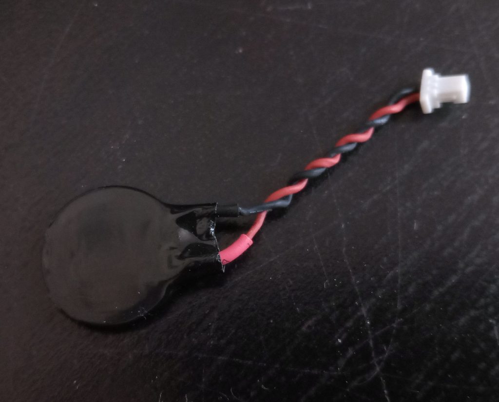
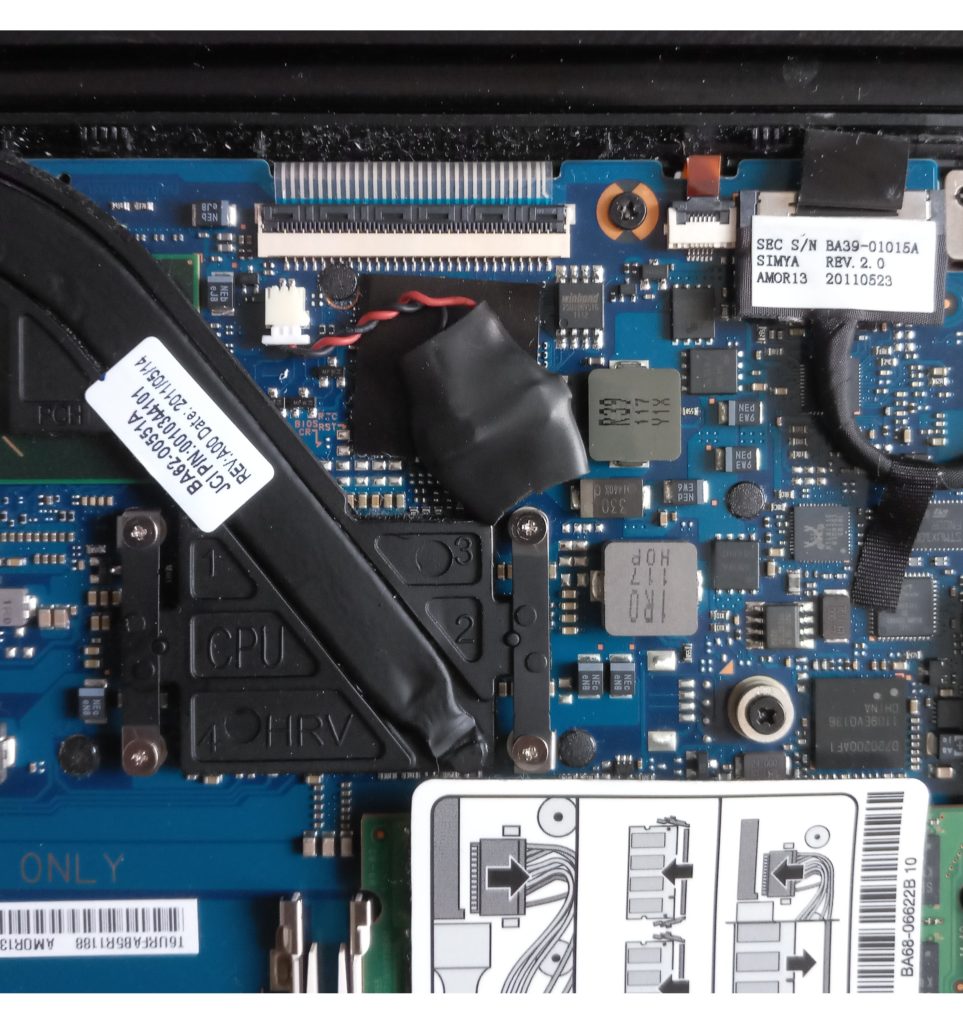
Here’s the culprit: Empty, unmarked

So, what about the battery? It’s obviously a coin cell on two wires with a plug. Nice idea, very accessible. Really. But at least some documentation would have been nice. No label, no print, nothing.

Measuring reveals: diameter 16 mm, thickness maybe a little below 2 mm. Hard to tell exactly while still in the rubber protection. So, could it just be a CR1616 or CR1620 cell with some spot welded soldering pins enclosed in some heat-shrink tubing?

No way to get the original part anymore. Samsung stopped selling laptops for quite a while in Germany (or even the whole EU, though it may have recently restarted again). Ebay has some offers. Anything from 5 to 150 € (seriously, it’s a coin cell, who charges more than 10 € for that?).

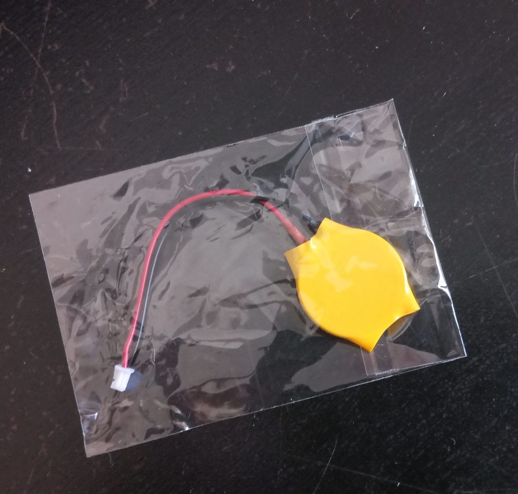
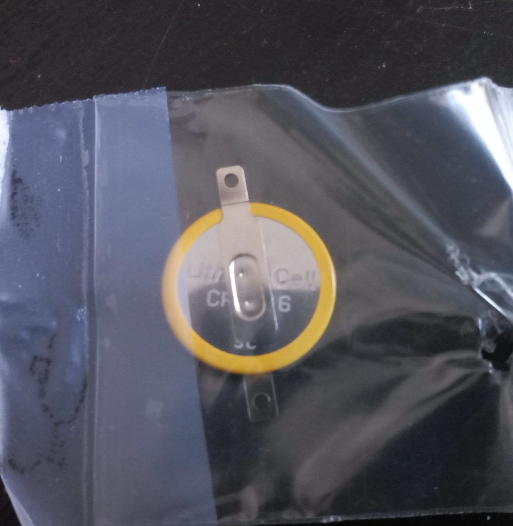
I decided to get one full package (cell, heat-shrink, wires and connector) for 5 € and a bare cell with spot welded solder pads for 2 €.

Got the wrong cell for 5 € (for a Samsung P20). Would’ve fit if it wasn’t for the connector.
CR1616 for 1,59 € to the rescue!

So, where’s the rant? Here:

COMPLEX ELECTRONIC DEVICES “BREAK” BECAUSE OF < 5 € COMPONENTS AND YOU NEED A F****ING PhD IN BATTERIES AND EBAY TO FIND REPLACEMENT PARTS BECAUSE NOONE THOUGHT OF PRINTING “CHECK UEFI SETTINGS” OR OF PRINTED LABELS ON A BATTERY OR A SIMPLE REMARK IN THE USER MANUAL (“YEAH, AND BTW, THE BATTERY IS A CR1616 FOR 84 CENTS WITH A MOLEX CONNECTOR, YOU’RE WELCOME.”)???

By now, this laptop would’ve been thrown out twice by every single average capable consumer in the world. And honestly, I cannot blame them. Right to repair will have a loooooong way to go.


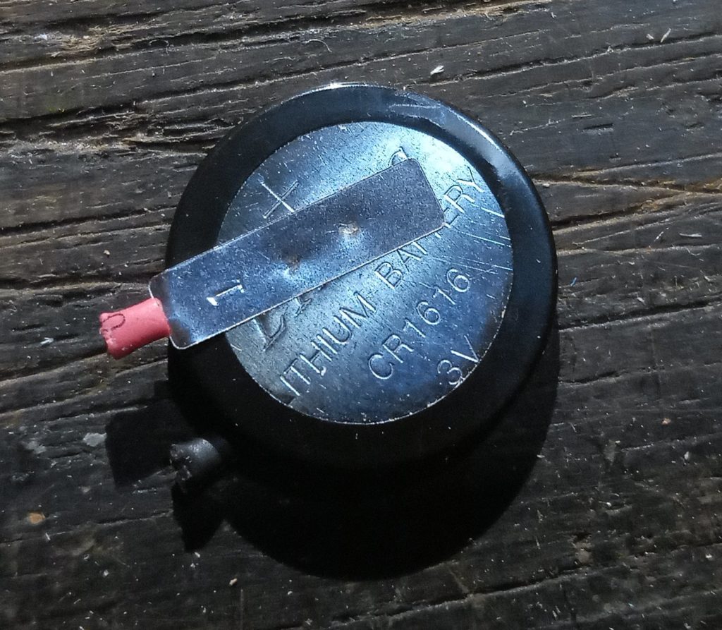
So yeah: Turns out the coin cell actually was a CR1616.

Cut off the wires, placed heat-shrink, soldered to replacement cell (not to the cell directly but to the solder tails), pack all in heat-shrink and voilà: a 1,65 € (+some solder and heat-shrink) replacement for a 10 year old laptop.

Categories
Uncategorized

A Toy Traffic Signal with an Arduino Nano

My kid likes traffic lights. So I decided to quickly build one. I started off on a breadboard with a bunch of components:

  • 3 × LEDs (red, amber, green)
  • 3 × 470 Ω Resistors (only had two, so the third are actually 2 1 kΩ in parallel)
  • 1 × 10 kΩ Resistor
  • 1 × Pushbutton Switch
  • 1 × Arduino Nano (actually a clone)

The circuitry is relatively simple. All LEDs’ cathodes point to ground (GND) through a 470 Ω resistor each to limit current and not blow anything. The anodes are connected individually to the digital port D3 through D5.

The button works such that, if open, it connects digital port D2 via a 10 kΩ resistor to the 3.3 V output of the Nano. When it closes, it’s supposed to pull D2 to GND, so it’s directly connected to it. The resistor serves to limit the current and – again – not blow anything.

That’s it. Now, for example, pulling D3 high (i.e. applying 3.3 V) will switch on the red LED. Likewise for D4 on the yellow and D5 on the green LED. Let’s introduce some human readable names instead of D2 through D5:

#include <Arduino.h>

#define BUTTON      D2
#define LED_RED     D3
#define LED_YELLOW  D4
#define LED_GREEN   D5

In the setup() function, I set the button pin as an input and the LED pins as outputs:

void setup() {
  pinMode(LED_RED, OUTPUT);
  pinMode(LED_YELLOW, OUTPUT);
  pinMode(LED_GREEN, OUTPUT);
  pinMode(BUTTON, INPUT);
}

To control the traffic light logic, I scribbled a Moore machine on a piece of paper, starting with a pedestrian traffic light (only red and green).

Moore machine with two states (red and green), initialised in the red state. Looped arrows indicate idle non-transition.

The machine starts in the red-light state. It remains there, unless the button is pressed. Then, it instantly switches to green (a pedestrian’s dream) where it remains until the button is pressed again.

This behaviour can be implemented by putting a simple switch case statement in the main loop() and implementing a state variable:

// States
enum states{ ST_R,
             ST_G
           }

void setState(bool red, bool green) {
  digitalWrite(LED_RED, red ? HIGH : LOW);
  digitalWrite(LED_GREEN, green ? HIGH : LOW);
}

void setRed() { setState(true, false); }
void setGreen() { setState(false, true); }

void loop() {
  switch(machineState) {
    case ST_R:
      // Serial.write("State: Red");
      setRed();
      break;
    case ST_G:
      // Serial.write("State: Green");
      setGreen();
      break;
}

Why use this enum thingy, you say? You could just use an int and call your states 0, 1, 2, etc., you say? Yes, you could also sign up for the biannual global brainfuck contest.

But, hey, wait, there are no transitions!

Exactly! For that purpose I’ll use an interrupt.

Just add one more function:

void ISR_ButtonToggle() {
  Serial.write("BUUUUTTON!\n");
  if(machineState == ST_R) {
    machineState = ST_G;
  } else if (machineState == ST_G) {
    machineState = ST_R;
  }
}

And don’t forget to actually bind the interrupt function in setup():

attachInterrupt(digitalPinToInterrupt(BUTTON), ISR_ButtonToggle, FALLING);

Now that’s a simple and pretty useless traffic light (well, I still like that I can switch it to green at will, this really should be the default pedestrian crossing light!).

But it is easy to extend. You want a yellow state? Add a yellow state ST_Y to your state machine (the switch case statement). Or you want it to show yellow before switching from green to red? Add a yellow-before-red state ST_Y_R. Or you really like to let people wait? Add a wait state. Oh, and of course you can call your states whatever you want.

Here is my full implementation of a non-pedestrian red-yellow-green traffic light as it is stated in the German traffic rules:

  • From red to green, with wait periods, go through
    • Red
    • Red+Yellow (yes, red+yellow, yellow meaning “get ready” and red meaning “not too fast, it’s still red, Freundchen!”)
    • Green
  • From green to red, with wait periods, go through
    • Green
    • Yellow (yes, only yellow. The meaning is disputed. Reasonable people say it means “Prepare to stop, if you can’t make it in time, it’s okay.” while idiots say it means “STEP ON THE GAS!”)
    • Red (This is also sometimes disputed, I won’t go into this.)
#include <Arduino.h>

#define BAUDRATE      9600
#define BUTTON        DD2
#define LED_RED       DD3
#define LED_YELLOW    DD4
#define LED_GREEN     DD5

// Transition delays
#define BLINK_WAIT        7
#define DELAY_R_RY        250
#define DELAY_RY_G        250
#define DELAY_G_Y         250
#define DELAY_Y_R         250
#define DELAY_R_G         250
#define DELAY_G_R         250

// States
enum states{ ST_R,
             ST_RY,
             ST_G,
             ST_Y,
             WAIT_R_RY,
             WAIT_RY_G,
             WAIT_G_Y,
             WAIT_Y_R,
             WAIT_G_R,
             WAIT_R_G };

states machineState = ST_R;
bool builtin_led = false;

void setState(bool red, bool yellow, bool green) {
  digitalWrite(LED_RED, red ? HIGH : LOW);
  digitalWrite(LED_YELLOW, yellow ? HIGH : LOW);
  digitalWrite(LED_GREEN, green ? HIGH : LOW);
}

void setRed() { setState(true, false, false); }
void setRedYellow() { setState(true, true, false); }
void setYellow() { setState(false, true, false); }
void setGreen() { setState(false, false, true); }

void blinkDelay(int delay_ms) {
  for(int i=0; i<BLINK_WAIT; i++){
    delay(delay_ms);
    digitalWrite(LED_BUILTIN, builtin_led);
    Serial.write(".");
    builtin_led = !builtin_led;
  }
  Serial.write("\n");
}

void ISR_ButtonToggle() {
  Serial.write("BUUUUTTON!\n");
  if(machineState == ST_R) {
    machineState = WAIT_R_RY;
  } else if (machineState == ST_G) {
    machineState = WAIT_G_Y;
  }
}

void setup() {
  pinMode(LED_BUILTIN, OUTPUT);
  pinMode(LED_RED, OUTPUT);
  pinMode(LED_YELLOW, OUTPUT);
  pinMode(LED_GREEN, OUTPUT);
  digitalWrite(LED_BUILTIN, LOW);
  digitalWrite(LED_RED, LOW);
  digitalWrite(LED_YELLOW, LOW);
  digitalWrite(LED_GREEN, LOW);
  pinMode(BUTTON, INPUT);

  attachInterrupt(digitalPinToInterrupt(BUTTON), ISR_ButtonToggle, FALLING);

  Serial.begin(BAUDRATE);
  Serial.write("Ready.\n");
}

void loop() {
  switch(machineState) {
    case ST_R:
      // Serial.write("State: Red");
      setRed();
      break;
    case ST_G:
      // Serial.write("State: Green");
      setGreen();
      break;
    case WAIT_R_RY:
      Serial.write("Wait: Red->RedYellow\n");
      blinkDelay(DELAY_R_RY);
      machineState = ST_RY;
      break;
    case ST_RY:
      setRedYellow();
      machineState = WAIT_RY_G;
      break;
    case WAIT_RY_G:
      Serial.write("Wait: RedYellow->Green\n");
      blinkDelay(DELAY_RY_G);
      machineState = ST_G;
      break;
    case WAIT_G_Y:
      Serial.write("Wait: Green->Yellow\n");
      blinkDelay(DELAY_G_Y);
      machineState = ST_Y;
      break;
    case ST_Y:
      setYellow();
      machineState = WAIT_Y_R;
      break;
    case WAIT_Y_R:
      Serial.write("Wait: Yellow->Red\n");
      blinkDelay(DELAY_Y_R);
      machineState = ST_R;
      break;
    case WAIT_R_G:
      Serial.write("Wait: Red->Green\n");
      blinkDelay(DELAY_R_G);
      machineState = ST_G;
      break;
    case WAIT_G_R:
      Serial.write("Wait: Green->Red");
      blinkDelay(DELAY_G_R);
      machineState = ST_R;
      break;
    default:
      Serial.write("Woops...\n");
      machineState = ST_R;
  }
}

Is this the best way to write this? Hell, no! Is it even a good tutorial? You tell me. I think it’s fairly simple and shows some evenly common concepts:

  • Using IO pins
  • Wiring LEDs without burning them or the output pin
  • Wiring a button*
  • Using #define statements to make code more readable and lives more easy
  • Using some abstraction (setState(), setRed(), etc.)
  • Using a state machine as an extensible concept
  • Using an interrupt (Why use an interrupt? Because it interrupts your code exactly when the button is pressed. It makes your little circuit very responsive and – at least in this example – it is even easier to write.)

*) You may encounter a problem that goes by the name “bouncing” (or in the beautiful German language “prellen”). That’s when your button press toggles multiple interrupts in a row. Try putting a capacitor in parallel with the resistor, or as a bad software hack, add a 5 ms delay (delay(5);) to the end of your interrupt function.

Anyways: My girl loves it. Ha! You thought she’d be a boy because it was a traffic light. Shame on you!

Categories
Finite Elements

Breaking Changes 2: Pygmsh, Fenics and Meshio>=4.0.0

Package versions this was tested with (2020-12-22):
gmsh 4.7.1
fenics 2019.1.0:latest
meshio 4.3.7
pygmsh 7.1.5

So, I thought, let’s do the article on Meshio>=4.0.0 and Fenics and show how interchangeable the gmsh itself, gmsh Python API, and pygmsh are. Well, I seem to not get it, but at least I did not manage to show that.

Using pygmsh with physical labels and Fenics is a bit unclear to me. I got it to work eventually, so here are the code blocks.

Generate the mesh using pygmsh

import pygmsh
# OpenCascade in pygmsh seems not to support extraction of lines from a rectangle (... to use with physical labels).
# So, let's use the geo kernel:
with pygmsh.geo.Geometry() as geom:
    r1 = geom.add_rectangle(0., 5e-3, 0., 2.5e-3, z=0.)
    geom.add_physical(r1.lines, label="1")
    geom.add_physical(r1.surface, label="2")

mesh = geom.generate_mesh(dim=2)
# We'll use gmsh format version 2.2 here, as there's a problem
# with writing nodes in the format version 4.1 here, that I cannot figure out
mesh.write("test.msh", file_format="gmsh22")

So, here’s the first oddity I would not get my head around: There seems to be no easy way to access the boundaries of the rectangle generated with the OpenCASCADE kernel. In gmsh’s API they were there as the first four one-dimensional items (although without the tutorial file there would have been no way I could have guessed that).

The second problem was writing the generated mesh to a gmsh format version 4.1, which resulted in an error message I could not quite track back:

>>> mesh.write("test.msh", file_format="gmsh") # That's gmsh41

---------------------------------------------------------------------------
WriteError                                Traceback (most recent call last)
  in 
      13 # with writing nodes in the format version 4.1 here, that I cannot
      14 # figure out
 ---> 15 mesh.write("test.msh", file_format="gmsh")
 /usr/local/lib/python3.6/dist-packages/meshio/_mesh.py in write(self, path_or_buf, file_format, **kwargs)
     158         from ._helpers import write
     159 
 --> 160         write(path_or_buf, self, file_format, **kwargs)
     161 
     162     def get_cells_type(self, cell_type):
 /usr/local/lib/python3.6/dist-packages/meshio/_helpers.py in write(filename, mesh, file_format, **kwargs)
     144 
     145     # Write
 --> 146     return writer(filename, mesh, **kwargs)
 /usr/local/lib/python3.6/dist-packages/meshio/gmsh/main.py in (f, m, **kwargs)
     109     {
     110         "gmsh22": lambda f, m, **kwargs: write(f, m, "2.2", **kwargs),
 --> 111         "gmsh": lambda f, m, **kwargs: write(f, m, "4.1", **kwargs),
     112     },
     113 )
 /usr/local/lib/python3.6/dist-packages/meshio/gmsh/main.py in write(filename, mesh, fmt_version, binary, float_fmt)
     100             )
     101 
 --> 102     writer.write(filename, mesh, binary=binary, float_fmt=float_fmt)
     103 
     104 
 /usr/local/lib/python3.6/dist-packages/meshio/gmsh/_gmsh41.py in write(filename, mesh, float_fmt, binary)
     356 
     357         _write_entities(fh, cells, tag_data, mesh.cell_sets, mesh.point_data, binary)
 --> 358         _write_nodes(fh, mesh.points, mesh.cells, mesh.point_data, float_fmt, binary)
     359         _write_elements(fh, cells, tag_data, binary)
     360         if mesh.gmsh_periodic is not None:
 /usr/local/lib/python3.6/dist-packages/meshio/gmsh/_gmsh41.py in _write_nodes(fh, points, cells, point_data, float_fmt, binary)
     609         if len(cells) != 1:
     610             raise WriteError(
 --> 611                 "Specify entity information to deal with more than one cell type"
     612             )
     613 
 WriteError: Specify entity information to deal with more than one cell type

Preparing mesh and boundary files for Fenics

Falling back to gmsh format version 2.2, I could generate the mesh and boundary files like in the original post:

outfile_mesh = f"{prefix:s}_mesh.xdmf"
outfile_boundary = f"{prefix:s}_boundaries.xdmf"

# read input from infile
inmsh = meshio.read(f"{prefix:s}.msh")
# delete third (obj=2) column (axis=1), this strips the z-component
outpoints = np.delete(arr=inmsh.points, obj=2, axis=1)

# create (two dimensional!) triangle mesh file
outmsh = meshio.Mesh(points=outpoints,
                      cells=[('triangle', inmsh.get_cells_type("triangle"))],
                      cell_data={'Subdomain': [inmsh.cell_data_dict['gmsh:physical']['triangle']]},
                      field_data=inmsh.field_data)

# write mesh to file
meshio.write(outfile_mesh, outmsh)
# create (two dimensional!) boundary data file
outboundary = meshio.Mesh(points=outpoints,
                           cells=[('line', inmsh.get_cells_type('line') )],
                           cell_data={'Boundary': [inmsh.cell_data_dict['gmsh:physical']['line']]},
                           field_data=inmsh.field_data)
# write boundary data to file
meshio.write(filename=outfile_boundary, mesh=outboundary)

Just to figure out that while pygmsh allows you to assign a string label to physical groups it numbers them automatically (apparently starting at 0). This is fine, it just seems to be written nowhere to be found.

Modifying the original code at the definition of the Dirichlet Boundary Condition did the trick (full listing at the end):

# ...

bcs = [
     do.DirichletBC(FS, do.Constant((0.0, 0.0)), outerwall, 0), # Choose physical group "index" zero here.
     ]

# ...

Conclusion

While this arguably still works and does the job it took me a few tries to figure out how. So, I hope this helps others at some point.

Full listing of the Fenics part

import dolfin as do
import numpy as np
import matplotlib.pyplot as plt

# Import Mesh
mesh = do.Mesh()
with do.XDMFFile(outfile_mesh) as meshfile, \
        do.XDMFFile(outfile_boundary) as boundaryfile:
    meshfile.read(mesh)
    mvc = do.MeshValueCollection("size_t", mesh, 2)
    boundaryfile.read(mvc, "Boundary")
    outerwall = do.MeshFunction("size_t", mesh, mvc)

do.plot(mesh); plt.show()

# Generate Function Space
FE = do.FiniteElement("RTE", mesh.ufl_cell(), 3)
FS = do.FunctionSpace(mesh, FE)

# Use markers for boundary conditions (watch for the change! ;-) )
bcs = [
    do.DirichletBC(FS, do.Constant((0.0, 0.0)), outerwall, 0), # Choose physical group "index" zero here.
    ]

# Trial and Test functions
E = do.TrialFunction(FS)
EE = do.TestFunction(FS)

# Helmholtz EVP (Ae = -k_co^2B*e)
a = do.inner(do.curl(E), do.curl(EE))*do.dx
b = do.inner(E, EE)*do.dx

# For EVP make use of PETSc and SLEPc
dummy = E[0]*do.dx
A = do.PETScMatrix()
B = do.PETScMatrix()

# Assemble System
do.assemble_system(a, dummy, bcs, A_tensor=A)
do.assemble_system(b, dummy, bcs, A_tensor=B)

# Apply Boundaries
[bc.apply(B) for bc in bcs]
[bc.apply(A) for bc in bcs]

# Let SLEPc solve that generalised EVP
solver = do.SLEPcEigenSolver(A, B)
solver.parameters["solver"] = "krylov-schur"
solver.parameters["tolerance"] = 1e-16
solver.parameters["problem_type"] = "gen_hermitian"
solver.parameters["spectrum"] = "target magnitude"
solver.parameters["spectral_transform"] = "shift-and-invert"
solver.parameters["spectral_shift"] = -(2.np.pi/10e-3)*2

neigs = 20
solver.solve(neigs)
print(f"Found {solver.get_number_converged():d} solutions.")

# Return the computed eigenvalues in a sorted array
computed_eigenvalues = []

for i in range(min(neigs, solver.get_number_converged())):
    r, _, fieldRe, fieldIm = solver.get_eigenpair(i) # ignore the imaginary part
    f = do.Function(FS)
    f.vector()[:] = fieldRe
    if np.abs(r) > 1.1:
        # With r = -gamma^2, find gamma = sqrt(-r)
        gamma = np.sqrt(r)
        do.plot(f); plt.title(f"{gamma:f}"); plt.show()
    computed_eigenvalues.append(r)

print(np.sort(np.array(computed_eigenvalues)))

Categories
Finite Elements

Breaking Changes: Fenics and Meshio>=4.0.0

Package versions this was tested with (2020-12-22):
gmsh 4.7.1
fenics 2019.1.0:latest
meshio 4.3.7
pygmsh 7.1.5

Check your versions with the code provided here.

Meshio is a great piece of software if you’re into converting meshes, or for that matter, if you’re using Fenics for finite elements calculations. However, the problem I experienced with both packages is their rapid development, consequently breaking changes and sometimes a lack of up-to-date documentation.

So, the Fenics community decided to embrace XDMF as mesh format of choice (good idea) but as usual with new stuff it’s WIP. So, there’s an ongoing thread on the discussion group which is extensive, but frankly hard to follow. After a day of fiddeling, I realised that a lot of example code discussed in the thread broke with Meshio version 4.0.0 and newer. It’s a subtle change in Meshio, which makes it non-obvious.

So, with no futher ado, here are code blocks that

  1. Generate a simple mesh using Gmsh
    1. A geo file
    2. A code block using Gmsh’s python API
  2. Convert msh-file to two XDMF files (mesh and boundary markers) for Fenics to digest
  3. Import of the XDMF files into Fenics and a minimal use-case

Generate a simple mesh using Gmsh

The three methods shown below are equivalent. Which one to choose depends on your workflow. It should be noted that getting the Gmsh Python API is not hard but still a bit tricky depending on context.

The goal is to build a rectangle of 5 mm × 2.5 mm with two physical groups (the boundary and the inner area).

Let’s start with the most static but straight-forward aproach: The geo-file straight from Gmsh’s UI. We’ll use the OpenCASCADE kernel (because, why not?):

SetFactory("OpenCASCADE");
Rectangle(1) = {-1.3, 0.5, 0, 5e-3, 2.5e-3, 0};
Physical Surface(2) = {1};
Physical Curve(1) = {1,2,3,4};

Save this file and generate a .msh file using the following command (we’re forcing a 2D mesh with -2 and gmsh format version 4.1 using -format msh41 here):

gmsh -2 -format msh41 test.geo test.msh

And last but not least using Gmsh’s Python API it looks like this:

import gmsh
import numpy as np

gmsh.initialize()
gmsh.model.add("test")
gmsh.logger.start()

r1 = gmsh.model.occ.addRectangle(0, 0, 0, 5e-3, 2.5e-3)
gmsh.model.occ.synchronize()

pg1 = gmsh.model.addPhysicalGroup(2, [1], tag=2) # inner surface
pg2 = gmsh.model.addPhysicalGroup(1, [1, 2, 3, 4], tag=1) # outer wall

gmsh.model.mesh.generate(dim=2)

gmsh.write("test.msh")

This example is closely based on an example in gmsh’s docs (t16.geo, t16.py). I would not say I’d know what gmsh.initialize, gmsh.model.add, gmsh.logger.start and gmsh.model.occ.synchronize actually do.

Convert msh-file to two XDMF files (mesh and boundary markers) for Fenics to digest

As I understand it, Fenics currently requires separate files for mesh and – let’s say – mesh annotations (like boundary names/numbers etc.). So, what the discussion came down to is converting the mesh as obtained from gmsh into two xdmf-files: test_mesh.xdmf and test_boundaries.xdmf.

The code below is shamelessly stolen mostly from dokken‘s post and Frankenstein-copy-pasted together with other contributions from forum users.

import meshio

# Let's introduce some symbolic names:
infile_mesh = "test.msh"
outfile_mesh = "test_mesh.xdmf"
outfile_boundary = "test_boundaries.xdmf"

# read input from infile
inmsh = meshio.read(infile_mesh)

# delete third (obj=2) column (axis=1), this strips the z-component
# outpoints = np.delete(arr=inmsh.points, obj=2, axis=1), create (two dimensional!) triangle mesh file
outmsh = meshio.Mesh(points=outpoints,
                      cells=[('triangle', inmsh.get_cells_type("triangle"))],
                      cell_data={'Subdomain': [inmsh.cell_data_dict['gmsh:physical']['triangle']]},
                      field_data=inmsh.field_data)

# write mesh to file
meshio.write(outfile_mesh, outmsh)

# create (two dimensional!) boundary data file
outboundary = meshio.Mesh(points=outpoints,
                           cells=[('line', inmsh.get_cells_type('line') )],
                           cell_data={'Boundary': [inmsh.cell_data_dict['gmsh:physical']['line']]},
                           field_data=inmsh.field_data)

# write boundary data to file
meshio.write(filename=outfile_boundary, mesh=outboundary)

So, after running this code snipped, you should see two files: test_mesh.xdmf and test_boundaries.xdmf

Import of the XDMF files into Fenics and a minimal use-case

Well, minimal may be something different. But since I’m using this approach for RF-related eigenvalue problems (EVP), this is as close to minimal as it gets:

import dolfin as do
import numpy as np
import matplotlib.pyplot as plt # for plotting mesh/results

# Import Mesh
mesh = do.Mesh()
with do.XDMFFile(outfile_mesh) as meshfile, \
        do.XDMFFile(outfile_boundary) as boundaryfile:
    meshfile.read(mesh)
    mvc = do.MeshValueCollection("size_t", mesh, 2)
    boundaryfile.read(mvc, "Boundary")
    outerwall = do.MeshFunction("size_t", mesh, mvc)

# Uncomment, if you want to see the mesh
# do.plot(mesh); plt.show()

# Generate Function Space
FE = do.FiniteElement("RTE", mesh.ufl_cell(), 1)
FS = do.FunctionSpace(mesh, FE)

# Use markers for boundary conditions
bcs = [
     do.DirichletBC(FS, do.Constant((0.0, 0.0)), outerwall, 1),
     ]

# Trial and Test functions
E = do.TrialFunction(FS)
EE = do.TestFunction(FS)

# Helmholtz EVP (Ae = -k_co^2B*e)
a = do.inner(do.curl(E), do.curl(EE))*do.dx
b = do.inner(E, EE)*do.dx

# For EVP make use of PETSc and SLEPc
dummy = E[0]*do.dx
A = do.PETScMatrix()
B = do.PETScMatrix()

# Assemble System
do.assemble_system(a, dummy, bcs, A_tensor=A)
do.assemble_system(b, dummy, bcs, A_tensor=B)
# Apply Boundaries
[bc.apply(B) for bc in bcs]
[bc.apply(A) for bc in bcs]

# Let SLEPc solve that generalised EVP
solver = do.SLEPcEigenSolver(A, B)
solver.parameters["solver"] = "krylov-schur"
solver.parameters["tolerance"] = 1e-16
solver.parameters["problem_type"] = "gen_hermitian"
solver.parameters["spectrum"] = "target magnitude"
solver.parameters["spectral_transform"] = "shift-and-invert"
solver.parameters["spectral_shift"] = -(2.np.pi/10e-3)*2

neigs = 10
solver.solve(neigs)

print(f"Found {solver.get_number_converged():d} solutions.")

# Return the computed eigenvalues in a sorted array
computed_eigenvalues = []

for i in range(min(neigs, solver.get_number_converged())):
    r, _, fieldRe, fieldIm = solver.get_eigenpair(i) # ignore the imaginary part
    f = do.Function(FS)
    f.vector()[:] = fieldRe

    if np.abs(r) > 1.1:
    # With r = k_co^2, find k_co = sqrt(r)
    k_co = np.sqrt(r)
    do.plot(f); plt.title(f"{gamma:f}"); plt.show()
    computed_eigenvalues.append(r)

print("All computed eigenvalues:")
print(np.sort(np.array(computed_eigenvalues)))

This gives me a 3 modes for this 5 mm by 2.5 mm waveguide and a bunch of spurious modes. That are filtered out because their k_co^2 is 1 or smaller.

Conclusion

This used to be easier (let’s say back in 2016). I’m fairly sure this is not the most efficient way (both programmatically and numerically) and I’m sure as well that there are better ways to solve this problem. For instance, instead of a generic triangular mesh a more structured triangular mesh or even a quad mesh would produce better solutions. Also, a higher order finite element should produce “smoother” solutions.

I also wanted to add a code block for pygmsh, but it turned out that there are a few catches with physical labels, how they’re numbered and labelled, and how to handle them in Fenics that I could not figure out. So, there’s a separate post on that here.

I am happy and thankful for any feedback!

How to check your package versions

import fenics
import meshio
import gmsh
import pygmsh

print("fenics:", fenics.__version__,
      "meshio:", meshio.__version__,
      "gmsh:", gmsh.__version__,
      "pygmsh:", pygmsh.__version__)