Numbers games: Z-Transform and some sympy

Back in uni me and control systems never really clicked. So I took a dive into the topic as I had the time. Long story short for all who know equally little or even less about the maths of control systems as I do:

Often, you model control systems using the Laplace transform. That’s nice and good for continuous systems.
Once you’re going to the discrete (digital) world, you want to use the Z-transform.
There is a (complicated) relation between Laplace domain and Z domain.
There are approximations, using a complex maps to map from Laplace to Z domain (a bilinear transformation, Tustin’s method, being the one used here).

This is a post on serendipity, because what this is about is actually neither control systems, Z-, or Laplace transforms but a numbers game. Bare with me.

Many systems can be modelled using a rational function of the form

$G(s) = \frac{\sum\limits_{i=0}^m \beta_i s^i}{\sum\limits_{i=0}^n \alpha_i s^i} \qquad\text{\alpha_0 = 1}$

You can easily put this into sympy and play around with it.

import sympy as sy

s, z, Ts = sy.symbols("s, z, T_s")

a0 = sy.S.One
a1, a2 = sy.symbols("alpha_1, alpha_2")
b0, b1, b2 = sy.symbols("beta_0, beta_1, beta_2")

G = (b0 * s**2 + b1 * s + b2) / (a0 * s**2 + a1 * s + a2)
G # use `print(sy.latex(G))` to get the LaTeX representation

$\frac{\beta_{0} s^{2} + \beta_{1} s + \beta_{2}}{\alpha_{1} s + \alpha_{2} + s^{2}}$

Nice. Let’s generalise this a little bit:

import sympy as sy

s, z, Ts = sy.symbols("s, z, T_s")

N, M = 2, 2

a = sy.symbols(f"alpha_1:{N+1}")
a = (sy.S.One, *a)
b = sy.symbols(f"beta_0:{M+1}")

G = sy.Add(*[b[i] * s**i for i in range(M+1)]) / sy.Add(*[a[i] * s**i for i in range(N+1)])

By playing with the values for N and M we can now generate any order of rational function we wish. Again, not the thing this article is about.

Then there is the bilinear transform called Tustin’s method that approximately maps the function G from the Laplace domain into the Z domain.

$s \Rightarrow \frac{2}{T_s} \frac{z-1}{z+1}$

Let’s do this in sympy:

tustin = 2/Ts * (z-1)/(z+1)

G.subs({s: tustin}).simplify()

$\frac{T_{s}^{2} \beta_{0} \left(z + 1\right)^{2} + 2 T_{s} \beta_{1} \left(z - 1\right) \left(z + 1\right) + 4 \beta_{2} \left(z - 1\right)^{2}}{T_{s}^{2} \left(z + 1\right)^{2} + 2 T_{s} \alpha_{1} \left(z - 1\right) \left(z + 1\right) + 4 \alpha_{2} \left(z - 1\right)^{2}}$

Sweet. Now, I want to have the representation in two polynomials in z (numerator and denominator) to extract the coefficients (because that’s what I wanted to hack into code):

num, den = G.as_numer_denom()
num = sy.Poly(num, z)
den = sy.Poly(den, z)

num.coeffs()
den.coeffs()

This gives you a nice, codeable result:

num: [  T_s**2*beta_0 + 2*T_s*beta_1  + 4*beta_2,
      2*T_s**2*beta_0                 - 8*beta_2,
        T_s**2*beta_0 - 2*T_s*beta_1  + 4*beta_2]
den: [  T_s**2        + 2*T_s*alpha_1 + 4*alpha_2,
      2*T_s**2                        - 8*alpha_2,
        T_s**2        - 2*T_s*alpha_1 + 4*alpha_2]

… but my eye spotted a pattern here. Do you see it? It’s easier to see in matrix representation, and I’ll only look at num (i.e. the expression with β_i in it, because I set ɑ₀ to 1):

$\text{num}^{(N=2)} = \begin{pmatrix} 1 & +2 & +4 \\ 2 & 0 & -8 \\ 1 & -2 & +4 \end{pmatrix} \cdot \begin{pmatrix} T_s^2 \beta_0 \\ T_s^1 \beta_1 \\ T_s^0 \beta_2 \end{pmatrix}$

Here is the resulting matrix for N = M = 3 and for N = M = 5:

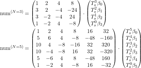
$\text{num}^{(N=3)} = \begin{pmatrix} 1 & 2 & 4 & 8 \\ 3 & 2 & -4 & -24 \\ 3 & -2 & -4 & 24 \\ 1 & -2 & 4 & -8 \\ \end{pmatrix} \cdot \begin{pmatrix} T_s^3 \beta_0 \\ T_s^2 \beta_1 \\ T_s^1 \beta_2 \\ T_s^0 \beta_3 \end{pmatrix} \\ \text{num}^{(N=5)} = \begin{pmatrix} 1 & 2 & 4 & 8 & 16 & 32 \\ 5 & 6 & 4 & -8 & -48 & -160 \\ 10 & 4 & -8 & -16 & 32 & 320 \\ 10 & -4 & -8 & 16 & 32 & -320 \\ 5 & -6 & 4 & 8 & -48 & 160 \\ 1 & -2 & 4 & -8 & 16 & -32 \end{pmatrix} \cdot \begin{pmatrix} T_s^5 \beta_0 \\ T_s^4 \beta_1 \\ T_s^3 \beta_2 \\ T_s^2 \beta_3 \\ T_s^1 \beta_4 \\ T_s^0 \beta_5 \end{pmatrix}$

Here are the resulting matrices for N = M = 4:

$\text{num}^{(N=4)} = \begin{pmatrix} 1 & 2 & 4 & 8 & 16 \\ 4 & 4 & 0 & -16 & -64 \\ 6 & 0 & -8 & 0 & 96 \\ 4 & -4 & 0 & 16 & -64 \\ 1 & -2 & 4 & -8 & 16 \end{pmatrix} \cdot \begin{pmatrix} T_s^4 \beta_0 \\ T_s^3 \beta_1 \\ T_s^2 \beta_2 \\ T_s^1 \beta_3 \\ T_s^0 \beta_4 \end{pmatrix}$

Here are the resulting matrices for N = M = 6

$\text{num}^{(N=6)} = \begin{pmatrix} 1 & 2 & 4 & 8 & 16 & 32 & 64 \\ 6 & 8 & 8 & 0 & -32 & -128 & -384 \\ 15 & 10 & -4 & -24 & -16 & 160 & 960 \\ 20 & 0 & -16 & 0 & 64 & 0 & -1280 \\ 15 & -10 & -4 & 24 & -16 & -160 & 960 \\ 6 & -8 & 8 & 0 & -32 & 128 & -384 \\ 1 & -2 & 4 & -8 & 16 & -32 & 64 \end{pmatrix} \cdot \begin{pmatrix} T_s^6 \beta_0 \\ T_s^5 \beta_1 \\ T_s^4 \beta_2 \\ T_s^3 \beta_3 \\ T_s^2 \beta_4 \\ T_s^1 \beta_5 \\ T_s^0 \beta_6 \end{pmatrix}$

The odd values for N and M produce matrices with all non-zero values, so I’ll look at those first.

What I find stunning is the fact that there are so many patterns and yet I fail to think of a pattern that creates the whole matrix. For example, the first column clearly follows the binomial distribution:

$\begin{pmatrix}N \\ k\end{pmatrix}$

where k is the row number starting with 0.

The first and last rows of the matrix are power series of 2 and -2 respectively:

$2^l \quad \text{and} \quad (-2)^l$

where l is the column number starting at 0.

Every column has a different sign pattern starting at all positive on column 0 and alternating, starting with + on the last column.

Ignoring the signs, the columns are related like this

N	#0 ↷ #N-1	#1 ↷ #N-2	#2 ↷ #N-3	#3 ↷ #N-4
3	྾ 8	྾ 2
5	྾ 32	྾ 8	྾ 2
7	྾ 128	྾ 32	྾ 8	྾ 2

What multiples relate the l^th column from the left with the l^th column from the right, ignoring the sign.

Maybe this follows from the power series mentioned earlier. But looking at the coefficients in each column the binomial pattern is lost as you move to the inside.

And last but not least wild zeros appear when you look at the even values for N and M:

Apparently, in the middle row as well as the middle column, every other value is zero.

All right, I’m absolutely sure mathematicians and control systems theoreticians have looked at this back in the day and this is all solved and done. Still, I found it interesting to look at.

If you want to create those values yourself, you can use this little script, and modify N and M. But beware, at N = 10 the script runs for 10 seconds.

import sympy as sy

s, z, Ts = sy.symbols("s, z, T_s")

N, M = 3, 3  # <-- Modify here

a = sy.symbols(f"alpha_1:{N+1}")
a = (sy.S.One, *a)
b = sy.symbols(f"beta_0:{M+1}")

G = sy.Add(*[b[i] * s**i for i in range(M+1)]) / sy.Add(*[a[i] * s**i for i in range(N+1)])

tustin = 2/Ts * (z-1)/(z+1)
G = G.subs({s: tustin}).simplify()

num, den = G.as_numer_denom()
num = sy.Poly(num, z)
den = sy.Poly(den, z)

for l in num.coeffs():
    p = sy.Poly(l, Ts)
    for i, B in enumerate(p.all_coeffs()):
        try:
            coeff, _ = B.as_two_terms()
        except:
            coeff = 0 if B is sy.S.Zero else 1
        print(f"{repr(coeff):6s} & ", end="")
    print()

Oh, and of course you can change N and M independently from each other, but I could not be bothered to look at this as well.